Measurements in Quantum Mechanics

Mathematics is undoubtedly a powerful key, essential to unlock our understanding of physics. However, maths alone would not get us very far, physics is a science and depends ultimately on empirical evidence obtained by observing what happens when we conduct experiments. Measurements are also an essential key to physics. A good mathematical model builds on prior observations and makes predictions of what we would observe in certain conditions - that is it predicts the results of experiments and what values we would actually measure. We rely on meters of various kinds and on making meters with the required degree of accuracy, however measurement in quantum mechanics takes on new meaning. It turns out that measurement is a very subtle thing indeed and often the results are far from expected by intuition alone.

In this article we look at some of the features and phenomena measured in quantum mechanics (QM) and delve deeply into what these measurements really mean. Be warned - Kansas is going bye-bye, to coin a phrase!

We begin with a simple experiment which will illustrate some of the theory we are going to need. The apparatus is illustrated in the circuit diagram below:

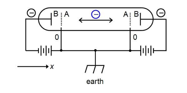
We have a sealed vacuum tube in which we have a single trapped electron that is free to move inside the tube. Electrons are negatively charged and our electron is indicated by the blue circle in the centre of the tube. At each end of the tube is a grid, A, held at zero potential (earthed to the equipment chassis). If the electron stays between these grids then it experiences no force (except for gravity which will be so slight on a particle so light that we will ignore it). However, the plates at B are negatively charged, so if the electron crosses either grid, A, then it suddenly becomes subject to a repulsive electric force (like charges repel). We make this force sufficiently strong to decelerate the electron and send it flying back into the middle of the tube (between A and A). The electron will tend to oscillate backwards and forwards. We have 'caged' our electron inside a 'box'.

Specifically, we have set-up an electric force-field to confine the electron. This force-field can be modeled as a one-dimensional (1D) potential energy well; 1D because the electron is only confined along teh x-axis (as indicated in the figure). We can represent this as follows:

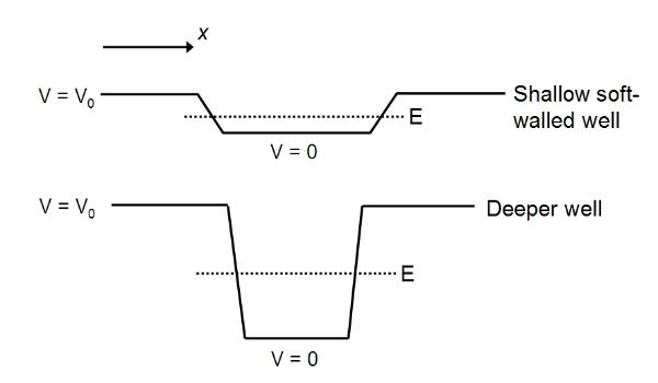
These are 1D square wells (of finite depth). V is the voltage (potential difference) which is a function of position x, being zero in the earthed centre of the box and rising steeply to our set potential (V=V0 at B) at the ends of the tube or walls of the well. The well at the top represents the force-field in the case when the repelling potential at B is quite weak: the well is shallow and 'has 'soft walls', that is the walls slope and are not rigid, which means in practice the electron can move through the walls a short distance (that is it can move past A a short way before being repulsed). The height of the well is proportional to the potential difference (between a and B) that is the strength of the force-field. If we increase the potential, that is strengthen the force-field, then the electron will be repulsed more strongly and more sharply: the walls are steeper and more rigid, and the well is also deeper. The greater the potential or force-field strength, the deeper the well. The deeper the well, the more vertical and more rigid its walls.

Note: our 1D finite square well potential is a simplified model of the force-field containing our electron. The same potential well can be used to model a range of situations, such as an electron bound to an atom. In this case, however, the square well is very inaccurate and is replaced by a Coulomb potential well, for the electrostatic force of attraction between the electron and the proton in say a hydrogen atom. More complexly shaped wells are harder to solve mathematically, and usually require a computer to approximate the mathematical solution to the required degree of accuracy. The square well, however, is a good example used in foundation QM courses, since it can be solved relatively easily by hand. Another elementary energy well is a parabolic well, which gives us the QM simple harmonic oscillator, which can be used to represent vibrating bonds in molecules.

If we increase our potential indefinitely, then our well will become infinitely deep and then its walls will be perfectly vertical and impenetrable. This is an ideal that can only approximate our experiment, but the so-called infinite square well is easier to handle mathematically than the finite square well and introduces many of the key features of quantum force fields. We can then calculate what possible energy values our electron might have. Consider many electrons in our box, or even better many boxes, each with one electron it, then it stands to reason that measuring the energy, velocity or momentum of the electrons will give us a well-defined average for a given potential, but what sorts of values would we obtain for the energy of an individual electron? 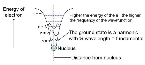Clearly this will vary statistically - not all the electrons will have exactly the same value. What is found is illustrated below:

Recall that a particle is also a wave, as a result of wave-particle duality. Our electron is a confined wave bouncing back and forth. In such a situation only certain frequencies of vibration are permissible, as the others cancel out, and the result is a standing wave. A similar result is obtained when a guitar string vibrates - only standing waves of certain frequencies occur, these are the harmonics, and the wave of lowest frequency (lowest energy and longest wavelength) is the fundamental. The frequencies of the other higher-energy harmonics are definite multiples of the fundamental. In our QM case the waves are solutions of the time-dependent Schrodinger wave equation (TDSWE) and are called wave functions. The square of the wave function corresponds to the wave pattern actually observed and the particle will be positioned somewhere on this wave. In fact we find that the time-dependent part disappears and the wave functions are solutions of the time-independent Schrodinger wave equation (TIDSWE) - like the guitar-string harmonics they are standing waves that do not change with time, they are stationary states or eigenstates. The wave functions
(eigenfunctions) are shown on the diagram above by the red curves. The blue horizontal lines correspond to the energy levels of each wave. There is an infinite number of such states inside the infinite well, called eigenstates, for the infinite well and each has its own discrete value for energy (the whole set of energies forming the set of energy eigenvalues). The fact that only certain discrete energies are allowed is the quantisation of energy. The total set of eigenstates is the spectrum of states. The lowest energy wave is the one nearest the 'bottom' of the well and this has the longest wavelength (it is the fundamental). Recall that for a photon in a light wave frequency and energy are linked by:

Where E is particle/wave energy, h is Planck's constant, and v (Greek nu) is frequency. This means that the lower the energy of the photon, the lower its frequency and the longer its wavelength (it is toward the red-end of the spectrum). A similar condition applies to our particle-waves - the lower the energy of the particle/wave, the lower its frequency and the longer its wavelength. Also for a light wave:

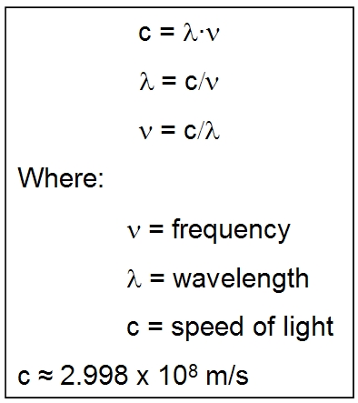
This applies to other waves, including particles, so long as we replace c by the speed of the wave.

Thus, the lowest energy state has the smallest frequency and the longest wavelength - it is the one at the bottom of the well with energy E = En = E1, the first eigenvalue (n = 1). Note that as we move to higher energy states (E2, E3, ...) the frequency increases by one half-cycle, the wavelength shortens and an extra half a wavelength occurs within the well. E1 is the ground state, and the other states are higher-energy or excited states.

Where is our particle?

A measurement of a particle in a potential well will reveal the particle to be in any one of the possible energy states or energy levels in the spectrum. Repeating the measurements on a large set of systems prepared in the same way, called an ensemble of states, will reveal that each state occurs with a given probability. Some will be more probable than others, some will be highly unlikely, but we can never determine beforehand which energy level (energy eigenstate) the particle will actually be found in. As for its position, it will be found somewhere within the space given by the square of the wavefunction. Where this squared wavefunction is zero (a node) the particle can never be found, and it will be most likely found where the square wavefunction is highest in amplitude. Again, we can never tell exactly where it will be until we measure it - there appears to be inherent indeterminacy in the system. Our particle seems elusive, having become more like a probability cloud. The best we can do, in principle as this is not apparently a practical limitation, is to state the
probability that a particle in a given system will be found in a certain region of space. We can also calculate average or expectation values for the various properties of the particle, such as its energy.

For those who are interested, the solution of Schrodinger's wave equation for the infinite well, including the derivation of the eigenfunctions and eigenvalues is shown in the series of thumbnails below.

The states for the finite square well can also be obtained by hand, though the calculation is a little more involved. A finite well has a finite number of eigenstates within it, but even the most shallow well always has at least one. The wave functions for the finite well also extend part-way through the 'soft' walls of the well before falling to zero (the particle can tunnel its way through the barrier) though we shall not consider the details of quantum tunneling here. This penetration of the walls, gives the particles slightly longer wavelengths than in the infinite well case and so slightly lower energies.

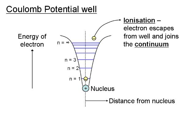
Bound and Unbound Solutions and the Continuum

So far we have looked at bound states, that is particles confined inside a force field or potential energy well. The deeper the well, the more bound states or energy levels it will have, though every well has at least one bound state, no matter how shallow. As the particle gains energy it jumps up to higher energy levels, until eventually it will jump out of the well altogether if given sufficient (kinetic) energy (energy at least equal to the depth of the well). If we had an infinite universe with just one energy well and one particle plus some energy source, then if the particle escapes from the well it would be in a region of empty space with no confining force fields to perturb it. It would be a free particle. Such a particle is then able to possess any amount of energy - it's energy is no longer quantised! Equivalently we can say that above the well, in free space, there is an infinite continuum of energy levels. In the real universe, there are always other particles and forces to interact with and no particle is ever truly free. However, a particle travelling through the 'void' of space would be relatively free and we still say that it exists in the continuum, except that the energy is still quantised, but such that there are so many close-spaced energy-states available to the particle that it belongs to a continuum to all intents and purposes. Such a particle is called a free particle, even though it is never entirely free. Such a continuum would exist, for example, in a rarified gas of atoms, in an approximate vacuum, and if enough energy is given to one of these atoms for one of its electrons to escape from the atom (this could be energy from a laser pulse or a collision with an electron beam, for example) then that electron becomes a free electron. The minimum amount of energy that must be given to the electron to achieve escape is called the ionisation energy of the atom. Ionisation energy depends on the atomic, molecular or ionic species from which the electron escapes.

Strong measurements

When we measure the position of our particle in a box, we find that it occupies any one of the energy level eigenstates, at 'random' (not strictly random as some states are more likely than others). These eigenstates are stationary and do not change with time. Once a measurement finds the particle in one state, it will remain in the same state on subsequent measurements or until the system is perturbed (the disturbance putting the system into a new state).

Actually, as Schrodinger's equation is linear and these are linear solutions, then just like any linear wave, we can add more waves together to form a new wave (superposition). This happens when we pluck a guitar string - the harmonics are superposed to give a note. We also see this in water waves: when they run into one-another they can cancel out or reinforce one-another as they add together. This means that our particle can be in a more general state that is a mixture of stationary eigenstates. Such a state gives us motion - an electron in a mixture of eigenstates can change with time, it can move and vibrate! This is how we go from standing waves to quantum motion. According to textbook QM the problem is that we can never actually observe the particle in one of these mixed states. Such states are fragile and as soon as we take a measurement we disturb the system, causing the mixed wavefunction to collapse into one of its component eigenstates. It is generally believed, or at least until recently, that a measurement inevitably collapses the system. This makes some sense, we are measuring something that is minutely small and we measure it by interacting with it. A good example is measuring the position of a photon in the two-slit diffraction experiment - we measure its position by intercepting it, causing it to collide with a screen! This is clearly quite drastic and is bound to alter the photon in some way. The result of the measurement then gives us the state of the photon after the measurement, when it has been brought to rest. These disruptive measurements are called strong measurements. We can only deduce the original mixed state in principle by analysing an ensemble of systems in the same initial state and seeing what proportion end up in each eigenstate, giving us the corresponding mixture.

Similarly, when an electron orbits the proton nucleus in a hydrogen atom, it is in a state of motion by virtue of the fact that it is in a mixed state, but as soon as we measure its energy or position it collapses into an eigenstate of the hydrogen atom, such as a 1s or a 2p or a 3d orbital, etc. Once in this state it does not orbit according to the maths, since it is in a stationary state. If it does orbit, then there are hidden variables that we can not measure and so know nothing about. As we shall see, the consensus opinion rules out such hidden variables, though the truth appears somewhat more subtle, as we shall see. Contradictions and confusions are already plentiful regarding this issue of electron orbits or trajectories.

Another example of a strong measurement is the Stern-Gerlach experiment which demonstrated the quantisation of angular momentum in atoms. An oven prepares a gas of alkali metal atoms, such as caesium (Cs) atoms. The intrinsic angular momentum of an atom depends on its electrons. Electrons can have spin angular momentum, due to their rotation, which can be pictured (though not literally!) as either clockwise or anticlockwise, or spin-up and spin-down, with an actual value of 1/2 (in units of Planck's constant over 2 x pi). Additionally, the electron can have orbital angular momentum, which happens when the orbital is not spherically symmetric, as in a p, d or f-orbital, but not the s-orbital which is spherically symmetric. In complete electron shells, the orbitals combine to give the shell spherical symmetry, so a complete shell has zero orbital angular momentum (the orbital angular momenta of the electrons in the shell cancel). In an orbital occupied by the maximum of 2 electrons, the electrons pair with anti-parallel (opposite) spins and so again the spin-angular momenta cancel. Again this means that in complete shells the net spin-angular momentum is also zero. In alkali metal atoms, the outer valence shell of electrons, the only incomplete shell, contains a single s-electron. Thus these atoms have no net orbital-angular momenta, but do possess a net spin-angular momentum of 1/2. When a measurement is made of the intrinsic angular momentum of these atoms only two possible values are found - either +1/2 or -1/2 (spin-up or spin-down) corresponding to the angular momentum of the single valence electron. These two values occur with equal probability (p = 0.5). Thus, the angular momentum of the atom is quantized - it can only take one of two possible values. In classic mechanics we would expect any value to be possible, within reasonable limits, as is the case for a spinning football, but this is not the case.

Note that, unless we invoke hidden variables, it is NOT generally the case that atoms possess either one or the other value prior to the measurement! Rather, the atoms usually possess a (linear) mixture or superposition of the spin-up and spin-down values, but as soon as the system is disturbed by taking a measurement, then each atom acquires one or other of the only two possible values. These two values are stable eigenstates. They are stationary states that do not change with time, so a repeated measurement on each atom would in this case produce the same result (unless the system is perturbed or allowed to evolve for sufficient time between measurements in which case it returns to a linear superposition of the two eigenstates).

In the Stern-Gerlach experiment, the cesium sample is vaporized in the oven and the emerging beam collimated to form a narrow beam in which all the atoms are traveling more-or-less in one direction (otherwise they do not pass through the holes in the collimators). This beam then passes through a pair of magnetic poles. These magnets are shaped so that the magnetic form between them is not uniform and so accelerates the atoms by deflecting them by an amount that is proportionate to the intrinsic angular momentum of the atoms (and to the strength of the field). Since there are only two such values, the beam splits into two and then strikes a screen or detector.

Above: the apparatus used in the Stern-Gerlach experiment. In reality, since the magnetic field weakens on either side of the beam, two arcs are formed, resulting in an approximate ellipse-shape as shown on the left-hand side of the diagram on the left. Classically we would expect any value within the range to occur, if the angular momentum of atoms was not quantized, in which case a solid ellipse would result as shown on the right-hand side of the diagram on the left.

• The Stern-Gerlach experiment demonstrates that the angular momentum of atoms is quantized.
  

• It also measures the spin angular momentum of a single electron when alkali metals are used.
  

Weak measurements

Strong measurements, as we have seen, disrupt the system being measured to such an extent that the system collapses into one of the possible eigenstates at 'random' (that is stochastically, some states may be more probable than others and so this is not strictly random, but which state results seems to be probablistic rather than deterministic). In a sense, the eigenstates or stationary states are the most stable and so when the atom system is strongly disturbed, or perturbed, it falls into one of these states. By this approach it is not possible to measure the original superposition of eigenstates directly. This is the state of affairs described in textbooks on quantum mechanics. However, recent experiments have shown that another type of measurement is possible - so-called weak measurements. In a weak measurement, the measurement perturbs the system so slightly that the particles do not collapse into an eigenstate, rather any change that occurs to them is reversible. However, this does not allow us to measure the superposed state of a single particle, such as an atom, because the weakness of the measurement means that very little information about the system is extracted. To counter this a large number or ensemble (population) of particles prepared in an identical manner must be used. This does not necessarily mean that we have to take an average of many experiments involving
one particle, though we could do it that way we can also use many particles and perform a single measurement to measure the so-called weak values to arbitrary accuracy. Thus, weak measurements describe the behaviour of ensembles rather than any particular particle.

For example, weak measurements to try and pin-point which path a photon follows in a double-slit diffraction experiment have yielded average trajectories along which the ensembles of photons travel, but not the trajectories traveled by individual photons - Heisenberg's Uncertainty Principle still forbids an individual particle from traveling along a precise trajectory since its energy and momentum can not, in principle, be both measured simultaneously with arbitrary position so we can not plot a graph of momentum versus time for a single particle! This would require hidden variables again - if the particles do indeed travel along precise trajectories, as some scientists think, then we still can not measure them, they remain hidden. As we shall see later the evidence is strongly against the idea of hidden variables, but does not rule it out completely. As we will explain later, I do not consider it more 'natural' to expect particles to follow precise trajectories and I do not think that intuition should be used to expect any particular behavior. Those that believe in definite particle trajectories adopt the idea is that since a football follows a definite trajectory then so should an electron
or atom, but I see no reason why we should expect this and indeed I consider this viewpoint at least as paradoxical as the more widely accepted interpretation given here as I will explain under the section 'Hidden variables'. Intuition simply fails us - the atomic and subatomic worlds are 'simply different'!

Several theoretical and practical methods have been devised for taking weak measurements. For example, to measure the movement (momentum) of an ensemble of charged particles, one could use a large charge attached to a sensor and measure the deflection of that charge (the momentum transferred to it by the electrostatic interaction). In the case of the double-slit experiment, scientists measured the polarisation of the photons, which weakly couples (is weakly dependent on) the momentum of the photons and so gives an imprecise measurement of the photon's momentum without changing its momentum irreversibly to any appreciable degree.

Another example, of relevance to quantum computing, uses a quantum point contact to measure electric charge. A quantum point contact is a narrow channel in a semiconductor between two metal electrodes (such as gold electrodes condensed onto the semiconductor base) indeed it is very narrow, typically of the order of one micrometre (one thousandth of a mm) or less. Such a narrow channel can make a very sensitive charge sensor, so that not much charge is needed to produce a reading. This is valuable when coupled to systems of qubits (quantum bits) used in a quantum computer. For example, a pair of qubits may consist of a pair of electron spins in a superposition state, in which the spins of the two electrons are entangled in a coherent state. A weak measurement is needed to read the qubit without destroying its coherence (causing decoherence) as a strong measurement would by forcing the coherent state or wavefunction to collapse into an eigenstate. The process is a little more subtle in practise (see our introduction to quantum computing for more details). In reality, rather than using a single pair of electrons, quantum dots are used. A quantum dot is a group of about one million semiconductor atoms, larger than a molecule, but much smaller than a
normal solid-state crystal or visible lump of matter.

A quantum dot can be used instead of a single electron or photon as a qubit. In a typical quantum dot, gold electrodes generate an electric field to confine a small number of electrons inside the quantum dot. A pair of such dots side-by-side can form a double quantum dot. Electrons within each dot interact weakly with the million or so nuclei (via the hyperfine interaction) and can interact with one-another to form a coherent state. Such a state can have a definite value of spin, since a coherent state behaves as a single quantum state. The two dots in a pair can then also be entangled into a single coherent state. Either the spin or the charge distribution in this dot-pair can be measured (for example if one excess electron is shared between the pair then different states exist depending which dot has the electron). The system must be kept very cool, since heat energy disrupts coherent states. Coherence is necessary for the computations to occur. One way to measure the spins of the two dots without destroying coherence is to measure it indirectly, via a third qubit linked to the other two. This third quantum dot is allowed to get warm, so that it acts as a sink for the entropy (disorder) caused by thermal effects. Electrons will slowly leak from the quantum dots by quantum tunneling. By using a sensitive detector, such as a quantum point contact, it is possible to measure this leaked charge whilst maintaining the state of the dots.

Optical systems of qubits are also possible, in which we deal with photon polarization rather than electron spin. Such a quantum dot was used as a source of single photons of well-defined wavelength in the double-slit diffraction experiment involving weak measurements.

The objective of a weak measurement is to transfer very little momentum from the system under study to the measuring apparatus, causing a minimum and reversible perturbation. This means that there are large uncertainties in the measurements, which can be reduced by studying a large number of identically prepared particles (an ensemble).

In contrast, strong measurements are more accurate (though limited in principle by the uncertainty principle) but do so by changing the momentum and state of the system irreversibly, in particular they remove any superposition (including entanglement and coherence) by placing the system in a stationary eigenstate. This also means that the state of the system prior to the measurement can not be measured in this way, only the final eigenstate. This is sometimes called post-selection, as the measurement returns the value the system has after the measurement! Atoms and subatomic particles are so minute and thus easily disturbed, that most measurements are of the strong type and weak measurements are a relatively recent realization.

The advantage of weak measurements is that they can yield information about a system prior to a strong measurement.

Hardy interferometers, the Hardy Paradox and more weak measurements

To further understand the issues of quantum measurements, we shall look at one particular gedanken (thought
experiment - an 'experiment' carried out in the mind by application of theory, typically prior to the techniques being available to actually perform the measurement). We can use photons of opposite phase or electron-positron pairs for this experiment, we chose the latter. Electrons and their positively charged anti-matter counterparts, positrons, can be generated as electron-positron pairs. electrons and positrons, like photons, exhibit wave-like behaviour and so can be used in an interferometer. An interferometer splits a beam of particles from a common source (which produces particles with a well-defined energy and wavelength) into two and directs these two beams along different paths before recombining them and measuring the resultant intensity. When two waves combine, they interfere with one-another by superposition (see our introduction to waves for a description of this). If the waves of the particles are exactly out of phase when they meet and combine then, just like water waves, they cancel out to produce nothing, a process called destructive interference. If, however, they are exactly in-phase then they recombine to give a wave of higher intensity (constructive interference). If the two path-lengths of the beams are identical then the two will generally meet in-phase and undergo constructive interference. (However, it should be noted that reflecting a wave, such as by bouncing it off a mirror, causes the phase to invert - crests become troughs and vice-versa). If the two path-lengths differ by exactly half a wavelength then the two destructively interfere. Differences of fractions of a half-wavelength will produce other results. In this way an interferometer can be used to measure distances with extreme accuracy.

In our experiment, we shall use a pair of interferometers, one for the electrons (e-) that are produced, another (which is identical to the first) for the positrons (e+). One such interferometer is shown below:

This is the one we shall use for the positron, as indicated by the + symbols. The positron beam is split into two by a beam splitter (BS) labelled BS1+. In the case of light this would consist of a half-silvered mirror that reflects half of the light whilst allowing the rest through. For charged particles we can use electrostatic deflectors. Each beam then bounces off a 'mirror' (such as a positively charged sheet) and the two sub-beams are recombined at a second beam-splitter (BS2+) before arriving at two detectors (A+ and B+). The arrows indicate the beam directions. The interferometer used for the electrons is identical, but with negative labels. Both are shown below:

It is possible to adjust the path-lengths of the two sub-beams (between BS1 and BS2) such that only the A-detectors (A+ and A-) will detect particles - particles headed for the B-detectors cancel by destructive interference (even a single particle, acting like a wave, can interfere with itself!). We shall fire a large number of electron-positron pairs into this system, one at a time. Whether each particle takes the inner or outer path is determined probabilistically - that is there is an equal chance that each particle will follow the inner path as the outer path and there is no way to predict this, other than to say that each path will be taken 50% of the time on average. What happens if we overlap the two interferometers such that their paths cross and interfere? Electrons and positrons will annihilate when they meet. As shown in the diagram below, we have overlapped the inner arms or paths of the two interferometers, leaving the outer paths as non-overlapping. This has two effects: 1) if the electron and positron both take the overlapping paths, then they will meet and destroy one-another. 2) Additionally, we can arrange things so that the paths interfere with one-another, whenever one of the particles is one of the overlapping paths, such that the self-interference of each particle is removed, allowing each particle, in principle, to reach the B-detector. E.g., if the electron is in the overlapping arm, it can interfere with the positron in such a way as to stop the positron interfering with itself, allowing the positron to reach detector B+.

What we would expect to happen?

• We might expect the positron to always arrive at the B+ detector whenever the electron arrives at the A-
  detector.
  

• We might expect the positron to arrive at the A+ detector whenever the electron arrives at the B- detector.
  

• We might not expect the positron to arrive at detector A+ whenever the electron arrives at A- as then the two should have crossed and annihilated instead!
  

• Suppose the electron arrives at B- and the positron at B+ ( a B+B- coincidence detection). We might suppose that the electron must have been in the overlapping arm, otherwise there would be no interference to offset the self-destructive interference of the positron. If the electron was not in the overlapping arm then the positron can not reach detector B+ (as was the case when the interferometers never overlapped).
  

• Similarly, when the electron arrives at B- and the positron at B+, we suppose that the positron must have been in the overlapping arm, otherwise it could not have interfered with the electron so as to prevent its destructive self-interference and so allow it to reach B-.
  

This then is the paradox: How can we have a B+B- coincidence detection in the first place, as both particles would have to have been in the overlapping arms and so should have annihilated one-another resulting in no detection at all.

Many would simply dismiss this and say that it's all theoretical, or that clearly the particles would annihilate and so a B+B- event could never be recorded. (We have assumed that the particles always annihilate when they meet). However, think about the original set-up. In the single interferometer, a single positron (or electron) could interfere with itself, preventing itself from reaching the B+ (or B-) detector. This is because of the wave nature of the particles - they can be in both paths at the same time!

For this reason, it is not so obvious that annihilation and hence no B+B- event could occur. We could attempt to resolve the paradox by making weak measurements on each path to determine whether or not the particles are in one or both paths. We couldn't use strong measurements as this would collapse the system and force the particles to be in one or other of the paths but never both.

Resolving the paradox?

What we could measure, by weak measurements, are the numbers of particles in each path (we have to use an ensemble of particle-antiparticle pairs to make weak measurements rather than a single particle-antiparticle pair). This situation can be analysed quantitatively, using quantum theory with number operators - mathematical operators that act on the mathematical representation of our system to extract the (average) numbers of electrons and positrons in each path.

Thus,
N(O+) gives us the number of positrons in the overlapping path;
N(NO+) the number of positrons in the non-overlapping path;
N(O-) the number of electrons in the overlapping path;
N(NO-) the number of electrons in the non-overlapping path;

In addition to these single-occupancy number operators, when the electron and positron are entangled in a coherent superposition, then we can also use the following paired occupancy operators:

N((NO+,NO-) gives the number of positrons and electrons in the non-overlapping paths;
N(O+,O-) gives the number of positrons and electrons in the overlapping paths;
N(NO+,O-) gives the number of positrons in the non-overlapping path and the number of electrons in the overlapping
path;
N(O+,NO-) the number of positrons in the overlapping path and the number of electrons in the non-overlapping path.

I wont give the calculations here, but the results for an observed B+B- coincidence detection are:

N(O+) = N(O-) = 1, so the electron and positron can indeed interfere with one-another;
N(NO+) = N(NO-) = 0;

N(O+,O-) = 0, so both were not in the overlapping arm and so did not annihilate;
N(NO+,O-) = 1 (pair), so the electron was in the overlapping arm, allowing the positron to reach B+;
N(O+,NO-) = 1 (pair), so the positron was in the overlapping arm, allowing the electron to reach B-;

N(NO+,NO-) = -1 (pair); this is very interesting since it means that the total number of electrons in the non-overlapping path is:

N(NO+,NO-) + N(O+,NO-) = -1 + 1 = 0;

Without this -1 value the number of particle-antiparticle pairs would be:
N(NO+,O-) + N(O+,NO-) = 1 + 1 = 2, which can not be since we are putting in one pair at a time!

Thus, the N(NO+,NO-) = -1 operator ensures conservation of total particle number, whilst the electron is allowed to reach B- at the same time the positron reaches B+ without annihilation!

Perhaps we should not dismiss Hardy's paradox after all. Perhaps it has given us an insight into how bizarre quantum mechanics can be! It also illustrates that weak measurements likely will not remove the 'oddities' of quantum mechanics, as some who adhere to the hidden variable theory might hope.

The full implications of weak measurements are not yet understood.

Atomic and molecular orbitals - are they real?

The wavefunctions (eigenfunctions) of the hydrogen atom represent the solutions to Schrodinger's wave equation for a Coulomb (electrostatic) potential or force field. We envisage the negatively charged electron as trapped inside the force-field of electrostatic attraction with the positively charged nucleus. These wavefunctions are the energy levels or orbitals of the electron in the atom, that is they describe the possible states of the electron. The energy of the electron depends primarily on how close to the nucleus it is and is given by the principal quantum number, n = 1, 2, 3, ... (a higher energy electron climbs up the well and so is further from the nucleus). The eigenvalues corresponding to these solutions represent the energy of an electron in the corresponding state described by the wavefunction and depend mainly on n. This is illustrated below:

Notice that n also corresponds to the number of nodes (points at which the displacement along the vertical axis is zero and thus where the wave cuts the horizontal axis) in the (radial) wavefunction (number of nodes = n - 1) - higher energy wavefunctions vibrate at a higher frequency and so have more nodes. The combination of nodes as determined by n and also the angular momentum of the electron determine the various shapes of the atomic orbitals (such as spherical s-orbitals, dumbbell-shaped  p-orbitals, etc.). Some of these shapes can be seen here. The pertinent question now is: Can we see atomic orbitals?

First of all, the eigenvalues can be verified by experiment as they account for atomic spectra which are very well understood. Schrodinger's model does have some simplifying assumptions, such as its failure to account for relativistic effects, but is still very accurate in predicting the eigenfunctions, and is extremely accurate when several corrections are made (such as incorporating relativistic effects).

Can we observe the wavefunctions? First of all, to be precise it is the square of the wavefunction we observe, since this corresponds to the charge density which is what we observe when we observe an electron. Of course these structures are too small to be 'seen' in the normal sense using light, but nevertheless are they real? Charge density can be measured in many ways and agrees with the predictions of quantum mechanics, but observing the radial structure and the nodes is a different matter. This would be like viewing an atom in cross-section.  It has been argued that wavefunctions are not real but are rather simply mathematical constructs.

The wavefunctions actually form an eigenbasis, essentially building blocks from which other states are made, by superposition. The eigenbasis depends on the choice of mathematical system used to describe the atom (position space or momentum space for example). Thus, we may end up building the same composite states from a different set of wavefunctions. Chemists will be familiar with the construction of d-orbitals from several eigenfunctions. However, some actual states are indeed described by single wavefunctions and so we must conclude that at least some of the wavefunctions correspond to real atomic shapes. However, eigenfunctions correspond to stable stationary states into which an initial wavefunction collapses after a typical strong measurement. The initial state is often a superposition of stationary states (a wave packet or mixture of wavefunctions in various proportions) so the initial mixed state usually elludes us (weak measurements possibly provide an exception to this).

This has been confirmed by recent experiments which use a photoionisation microscope to view the 'nodal structure' of hydrogen atom wavefunctions almost directly. Not every state of an atom can be observed so directly, but hydrogen atoms have been prepared in Rydberg states, that is in high energy states by applying lasers and then placed in an electric field. Rydberg atoms are large distended atoms (up to one hundredth of a millimetre in diameter, or about the size of a 'typical' animal cell!) and so easily distorted by relatively weak magnetic fields. This distorts the atom in a direction determined by the field, such that instead of states described by n, we now have states described by n1 and n2, in which n2 can be large (e.g. n2 = 28, a Rydberg state) whilst n1 can be small (n1 = 0, 1, 2, 3, 4, etc.). An atom distorted by an electric field in this manner is in a Stark state and the change to its wavefunctions and eigenvalues is the Stark effect. Now, Rydberg atoms are unstable, lasting about one second before shrinking by losing an electron (causing 'n' to reduce) but the electric field can be arranged to act as a barrier to the electron's escape. However, electrons will sometimes quantum tunnel through this barrier and escape, as the atom becomes ionised (the electron can be described as quasi-bound). As it happens, calculations show that , remarkably, the tunneling electrons in this case, tunneling from an ensemble of similar atoms, carry information about the nodal structure of the wavefunctions (n1 specifically) with them, as predicted by calculation. These patterns are very similar to the 1s, 2s, 3s and 4s orbitals in form (though not quite identical as these are Stark states). More precisely, these experiments prepared the atoms in a superposition of stationary states, but the wave packet collapses into one eigenfunction following (strong) measurement. The results of these experiments are discussed here: http://physicsworld.com/cws/article/news/2013/may/23/quantum-microscope-peers-into-the-
hydrogen-atom

It is worth mentioning that a number of other experiments have given insight into the structure of wavefunctions in both individual atoms and molecules. In molecules, molecular orbitals form as the result of combination of certain wavefunctions in the constituent atoms (at least approximately). A recent experiment with an atomic-force microscope, a device which passes a very tiny probe over a surface and measures the force acting on the probe due to interactions such as covalent bonding or quantum tunneling, gave a good visualization of what appears to be a hybrid orbital between a 3s atomic orbital and two 3p atomic orbitals consisting of two hemispherical lobes. Additional experiments with carbon chains have given a good direct visualization of the orbitals, which although molecular rather than atomic orbitals, have strong atomic character in the end atom. These experiments confirmed the s and p nature of these orbitals: Imaging_the_atomic_orbitals_of_carbon_atomic_chains_with_field-emission_electron_microscopy.pdf.

Those with a chemistry background may be familiar with the shapes of the p, d and f orbitals presented in chemistry texts, for example the three dumbbell-shaped p-orbitals which are identical to one-another in shape but lie along different axes (they are at right-angles to one-another). However, these do not correspond to the shapes of the eigenfunctions (stationary states) obtained by solving Schrodinger's equation for the hydrogen atom (see: mathematical plots of the atomic orbitals). Why the discrepancy? First of all, mathematically speaking, any linearly weighted sum of eigenfunctions is also a solution to Schrodinger's equation. Thus, we can, for example, add one-quarter of an s-orbital to 3 quarters of a p-orbital and obtain an acceptable solution. However, such superpositions are no-longer stationary states (the electron can undergo wave-motion as an oscillating wave packet) and any strong measurement performed on our hybrid orbital will cause it to collapse into either the s or p state: it will not remain in a superposition after a strong measurement. What is done to construct the standard orbitals shown in chemistry books is to apply superposition, but only to the spherical harmonics. The spherical harmonics are combined in such a way that the imaginary component disappears to obtain real (i.e. non-complex) spherical harmonics (it is not clear why this is done, since squaring the wavefunction to obtain the probability distribution abolishes the imaginary part anyway). In this way a new set of basis states (eigenstates) are obtained.

The end result, for the p-orbitals at least, is that each p-orbital becomes equivalent: they each have the same shape but in a different orientation. This perhaps makes sense when you consider that chemists are concerned with atoms surrounded by other atoms in molecules. Consider an atom in a solid crystal, for example, it is surrounded by magnetic fields on all sides and if the crystal is isotropic (uniform in each direction) then there is no reason to suppose the orbital;s will have a preferred shape along any one axis, as is the case with the H atom eigenfunctions given in physics texts. We might expect the p-orbitals to combine in some way to equalize themselves. Some authors dismiss the whole maneuver as inappropriate. Personally, I also have my doubts, but I am not prepared to dismiss this approach in the absence of empirical data. It is important, therefore, to carry out measurements on the shapes of atomic orbitals, wherever possible, to verify which solutions of Schrodinger's equation give the correct eigenstates.

Let us look at another two-state system: photon polarization (we could just as easily stick with spin which is also a two-state system with spin-up and spin-down). Light can exist in one of two polarization states: horizontally polarized (H) and vertically polarized (V) with respects to the orientation of a polarizer. Such a polarizer might consist of a calcite crystal. A beam of light, initially consisting of light waves of all polarizations, emerging from a polarizer will contain just two polarizations: horizontal and vertical. 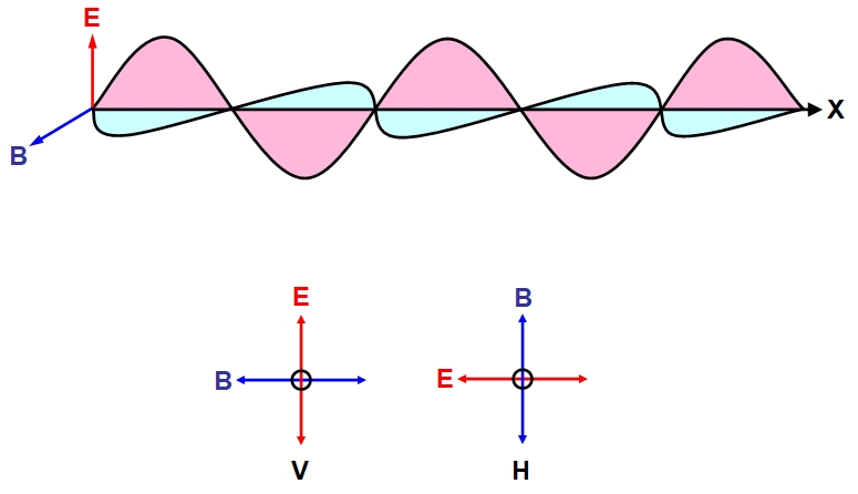What does this mean? Classically we can think of a light wave as consisting of oscillating electric and magnetic fields, each oscillating perpendicular (at right-angles to) to the other and both oscillating perpendicular to the direction of motion of the wave (or ray or beam) of light. This is illustrated below for a ray of light moving in the direction of the positive x-axis (from left to right) with the electric field (E) shown in red and represented as a vector, and the magnetic field in blue represented by the vector B. Underneath we view the ray head-on and depict two waves of opposite polarity: the polarity is, by convention, determined by E, which oscillates along the vertical plane in the vertically polarized wave (V, bottom left) and oscillates horizontally in the horizontally polarized wave H (bottom right).

Light waves radiating from a variety of natural sources, including the Sun, are unpolarized consisting of a mixture of light waves in which the electric vector points in a random direction from 0 to 360 degrees perpendicular to the direction of motion (note B is always perpendicular to E). Upon passing through a polarizer, such as a calcite crystal, the light interacts with the vibrating ions in the crystal lattice and emerges with definite planes of polarization (the plane of polarization refers to the plane formed by E and the direction of wave motion). If we measure this polarization then we find that 50% of the waves are H polarized, 50% v polarized. this kind of polarization. this is illustrated schematically below: HV representing our polarizer and measurements occurring on the right-hand side of the polarization of emerging light.

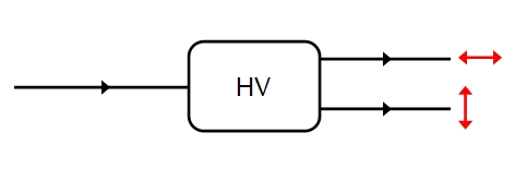
This type of polarization is called linear polarization or plane polarization. It is possible to polarize light in other waves: in circularly polarized light E rotates either clockwise or anticlockwise about the direction of wave propagation with E retaining a constant amplitude and rotating at a constant rate. The key point is that only two mutually exclusive states are being considered. The top output channel will represent H in these diagrams, the bottom channel V.

So far the discussion has been classical, using an electromagnetic wave representation of light. However, if we dim the source of the light until it emits only one photon at a time then we will still find that 50% of the photons are H polarized, 50% v polarized, on average. For any individual photon, however, the polarization is random: this is a stochastic process (unless we assume hidden variables). Recall that we are not saying that a photon leaves the source either H or V polarized: the source emits photons of no particular polarization, instead we are saying that the photon has no definite polarization until it is measured (according to the Copenhagen interpretation of quantum mechanics which is the most widely accepted). Instead we think of a photon as so minute that any act of (strong) measurement, which requires an apparatus to interact with the photon, changes the state of the photon - it is perturbed by the measurement and what we obtain is the polarization after the measurement, which collapses into either H or V with equal probability. However, there is one situation in which we can know the value before measurement: H and V are eigenstates (the only two possible eigenstates) that is they are stationary states, so if we measure the polarization of the photon and find it is H, and repeat the measurement on the same photon, then it will remain H as long as the measurement is carried out within a short enough space of time. The photon has a natural tendency to drift back into an undecided state ( a superposition of eigenstates) and once in this superposition of H and V (basically H and V simultaneously, or equivalently neither H or V) a measurement can result in either H or V with 50:50 odds. However, if we repeat the measurement before the photon drifts into this uncertain state then a repeated measurement will always yield the same eigenstate as the previous measurement. A measurement will always collapse the photon into an eigenstate of the property or 'observable' being measured. Each eigenstate has an associated eigenvalue and the eigenvalue is what is actually measured: the eigenvalue represents an eigenstate. (In some systems more than one eigenstate may have the same eigenvalue, and these are called degenerate states, but that does not apply to this example). This is illustrated below:

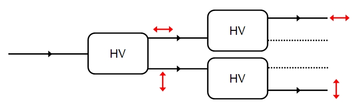
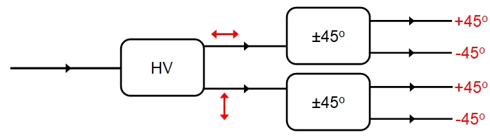
Now, space has no unique horizontal or vertical direction!the eigenstates H and V are only relative to the orientation of our polarizer (our calcite crystal). If we orient the polarizer at 45 degrees then we are now measuring polarisation with respects to the new orientation and our eigenstates will be +45 and -45, or whatever we want to call them, and neither H nor V will be an eigenstate of the new measurement. What this means is even if we separate the H and V photons coming from the HV polarizer (e.g. by using a polaroid to block out one or the other) then we can say nothing about the new state with respects to 45-degrees prior to measurement: both H and V photons give readings of +45 and -45 with equal probability. Again, this is random for any individual photon, but by the law of averages 50%, on average, will be +45, 50% -45 whether we start with H or V photons. It seems we have given the photons a new polarization property. Furthermore, if we took either the +45 or the -45 photons and passed them back through a HV polarizer, then on average 50% would emerge as H, 50% as V: the original H/V polarization no longer applies!

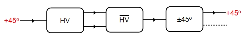
Wait a moment though! Things are not quite so simple! If we pass, say the +45 photons through a HV polarizer and then pass both the resultant H and V photons that emerge through a second polarizer which is reversed (indicated with an overline as HV) then the initial H/V polarization is undone and we end up back with an unpolarized beam. If we then measure the 45-degree polarization then we will find that it is always +45. On the face of it this would appear to lend support to the hidden variable idea that each photon has definite H/V and +45/-45 degree states, but ...

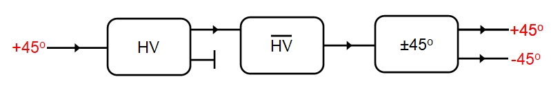
The Copenhagen interpretation, that photons have no definite polarization until such has been measured has not been violated! The problem is the photons passing through the first HV polarizer were not actually measured but simply passed through from HV to HV and were only measured at the end, when we find that, according to teh previous rules, they remain in a +45 eigenstate. instead if we measure the polarization of each photon as it emerges from HV, so that it enters HV with a definite H or V eigenstate then the final measurement will yield either +45 or -45 with 50:50 odds - the original H or V eiegenstate has been lost and the photon changed to +45 or -45 polarization at random! It would seem there is something special about measurements, and that is an issue we will return to later.

Quantum Entanglement

One of the most striking departures from the logic of classical physics and that of quantum mechanics is the phenomenon of etanglement. Consider two electrons, for example, one spin-up, the other spin-down:

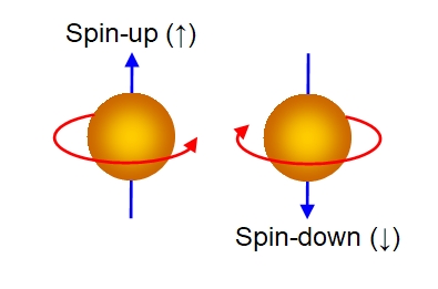
Here we have used a classical representation by visualizing the electrons as spinning balls with the direction of rotation (clockwise or anticlockwise) determining the spin direction. Electrons aren't really like this, but they do have a quantum property called spin which in some ways is like a quantum equivalent of spin angular momentum. Electrons are of course impossible to visualize correctly. The quantum number spin (s) takes values of +½ or -½ (in units of ℏ = Plancks constant divided by 2π) with reference to any particular direction. Space of course has no preferred direction, but here we have taken it to be the vertical direction; for example, we could have the electrons in the presence of a vertically aligned magnetic field, which would impose this direction upon them.

If far apart from one-another then our two electrons behave independently and we can describe their collective state mathematically as a product state: the state of one electron multiplied by the other. (This means that the two individual states factorize out from the combined state - in other words they are independent of each other). For example spin-up multiplied by spin-down: combined product state = ↑ x ↓.

However, if brought sufficiently close to one-another then the wavefunctions describing their states (giving us the probabilities of finding each electron as spin-up or spin-down) overlap and the two electrons become indistinguishable: they function as a single two-electron entity. This happens in the helium atom, for example, which has only two electrons. Their wavefunctions  have become entangled. Focusing on the wavefunctions describing their spins (spin wavefunctions) we can represent the electron spins as a singlet state or a triplet state, both of which are entangled. Let us assume they retain their opposite spins and are in a singlet state (since this is mathematically and conceptually simpler than the triplet state). The wavefunction of the spin singlet can be written as:

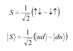
Where the top and bottom equations are two alternative ways of representing the same thing (two different commonly used notations): the bottom equation uses Dirac's bra-ket notation. The first arrow represents the first electron and the second arrow represents the second electron, though in truth they are now indistinguishable since both have a certain character of up-ness and down-ness. This singlet state is an entangled state - we can not tease out the spin of one electron and multiply it by the spin of the other - this is NOT a product state (it will not factorize) but an entangled state. Actually it is a maximally entangled state (in general there is a spectrum of variously entangled states between product states and maximally entangled states.

The interesting thing about entangled states is that we can know all there is to know about the entangled state and yet be unable to know anything about the states of its component parts - the two electrons really have lost their individual identities. If we try to learn more by measuring the spin of one of the electrons (in the vertical direction), then the entanglement unravels as the wavefunction collapses (into a spin eigenstate, a state of definite spin, either up or down): we will find that the electron is either spin-up or spin-down (with equal probability). However, the spins of the two electrons are correlated: once we know the spin of one electron we will know with certainty that the other electron has the opposite spin, even without measuring it!

Interestingly, if we separate the two electrons without measuring the spin of either (as soon as we do the wavefunction collapses) then no matter how far apart the electrons are as soon as we measure the spin of one, we know the state of the other electron's spin! This has led to claims that this represents 'spooky action at a distance'. In a way it is, but contrary to what is often stated it does NOT violate the causality of relativity. What we are saying is that supposing one of the electrons was given to Alice and the other to Bob, without disturbing (measuring) them, and they flew several light-years apart in their spaceships and then Bob measures the spin of his electron and finds it to be up. He immediately knows the spin of Alice's electron: down. sure enough if Alice then measured her electron's spin she would see that it is indeed down. However, Bob could have measured his electron as down, with equal probability (we could imagine an ensemble of many such electron pairs in singlet states to make a statistically valid experiment) in which case Alice would measure hers as up. If they had many such separated singlet states and measured away, then every time Bob finds down, Alice finds up. Every time Alice finds down, Bob finds up, and vice-versa. Each, however, would obtain 50% up spins and 50% down spins, on average, as if with random probability of finding spin up or spin down each time. Neither Alice or Bob can notice anything odd about their measurements: the spin measurement appears truly random giving spin-up or spin-down in a random pattern with equal odds. It is only after they share their results with one-another that they will see the correlation: whoever measured the spin of any given entangled pair first, would determine the spin measured by the other.

So what? You may think! This would be expected if each electron had a definite spin all along and they were randomly shared out between Alice and Bob. However, this invokes hidden variables: the assumption that a particle has definite properties before we measure them. However, this violates the Copenhagen interpretation in which measurements change the properties of a particle, as we saw them apparently do above with photon polarization. The Copenhagen interpretation states that neither electron had a definite spin until the measurement was carried out and it acquires either spin-up or spin-down randomly. Einstein was in favor of hidden variables and was not keen on 'spooky action at a distance' nor on the inherent randomness of the Copenhagen interpretation (even though he contributed so much to the quantum physics that gave rise to both concepts!). We shall say more about hidden-variable theories and why these are not largely accepted, later. Let us stick with the idea of the Copenhagen interpretation for now. we are assuming that neither electron had a definite spin-state before a measurement was carried out. Furthermore, measuring either one of the electrons gives it a spin-state, up or down, at random but the other electron acquires the opposite spin-state instantaneously no matter how far away it is. in a sense some kind of instantaneous 'signal' has passed from the measured electron to its partner, 'informing' it that a measurement has taken place.

The problem is, if signals can be sent faster than the speed of light, then according to Einstein's theory of Relativity, causality can be violated: it would be possible to learn of an event before it took place! (This is not intuitively obvious but follows as a logical consequence of relativity theory). No signal can travel faster than light without the order of time getting messed up! Assuming time can not be messed up in this way then how do we explain this 'spooky action at a distance'. The answer is thus: entanglement can not be used to send any meaningful signal. Alice's measurements may correlate with Bob's but neither notices anything untoward: each obtains the results they expected in the absence of entanglement, even though they can tell and know that the state is entangled. It is only when they send their results to one-another and compare notes that they can see the correlation. This requires, say, Bob to signal Alice that a measurement on a given entangled pair has taken place, then she can know the state of her electron before she measures it. However, Bob has no known way to send his results faster than light. Therefore, causality is not violated and neither is Relativity. (Whether or not physics eventually finds a way to send meaningful signals faster than light is another matter. Currently, this does not seem possible in principle). 'Spooky action at a distance' does not (currently and in principle) allow us to send signals (carrying an encoded message) faster than light.

Testing for entanglement - the density matrix

In quantum mechanics a density matrix is a matrix of probabilities for a discrete system like spin (or probability densities for continuous random variables). For example for the entangled singlet the density matrix (of the whole system of both spins) is compared below to that for a product state in which both electrons are equally likely to be spin-up or spin-down:

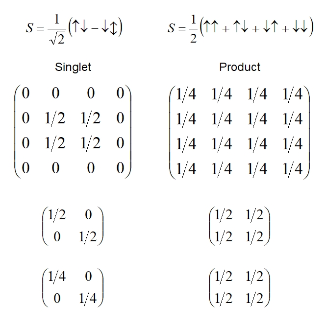
Above: from top to bottom - the spin sate, density matrix of the two-electron system, density matrix of the one electron subsystem, one-electron density matrix squared; for both an entangled and a product state.

To be precise, the leading diagonal (from top left to bottom right) gives us the probabilities. The top matrix in each case is the density matrix for the entire combined state. Notice that both leading diagonals add up to one, as the total probability of all possible outcomes must be one (certainty). We say that the trace of the matrix (sum of the elements on the leading diagonal) is equal to one in both cases. Furthermore, each of these matrices is equal to its own square (if you know matrix algebra then you can check this by multiplying each density matrix by itself) and the trace of the squared matrix is also one. These two facts tell us that we are dealing with pure states in both cases, as opposed to mixed states in which contributions arise from another state (such as a third entangled electron we forgot about): entangled states are pure states when we consider the entire system. Note the subtlety of this definition of 'mixed state' which differs from a more colloquial use of 'mixed' to refer to a superposition of states - superpositions can be entangled or product states and both are pure when we consider the whole system, that is:

The density matrix is equal to its own square and the trace of the squared density matrix = 1. This defines a pure state.

(Usage of the terms 'pure' and 'mixed' may not always be consistent and the usage should be checked in any particular text).

The second matrix gives a subsystem of the state. It gives the density matrix for just one electron from the two-electron system. Considering just one electron as a system in its own right we find that for the product state the density matrix equals the squared density matrix (shown as the third matrix at the bottom) and its trace equals one - in other words the one-electron subsystem for the product state is also a pure state. Thus the two states factorize into two distinct states and we can consider each electron individually and know all there is, in principle, to know about it. This is to be expected since the two electrons are not influencing one-another.

However, the subsystem of the entangled singlet state gives a density matrix that is not equal to its own squared matrix and the trace of the density-squared matrix is less than one. This defines a mixed state.

This is to be expected: when considering one electron in an entangled pair we find that we only have part of a system - the single electron can not be treated as a whole system in its own right - but is part of a mixed state.

There is another easy way to test for entanglement, which we wont go into here: we can calculate the correlation between the two one-electron subsystems - if they correlate with one-another then the system is entangled.

Entanglement of particle spins (or qubits) forms the basis of quantum computing.

Example - entanglement of two diamonds at room temperature

With some knowledge of density matrices we can better understand a noted experiment published by Lee et al. in 2011 in their paper: Entangling Macroscopic Diamonds at Room temperature. Entanglement is easily disrupted by thermal noise and so entangled systems are generally cooled to very low temperatures for experimental purposes. There is more thermal noise in larger systems so entanglement is generally only readily observed on submicroscopic systems, such as cold electrons. This poses practical problems for the construction of quantum computers. Entanglement is also being increasingly suspected to play important roles in biological systems (and there is evidence for this). For these reasons there is considerable interest in entanglement in 'warm' systems at room temperature.

In their experiment, Lee et al., took two diamonds, 3 mm in diameter that were 15 cm apart. The advantage of using diamond is that the covalent bonds are very strong and this creates a stiff lattice that is less effected by thermal noise, making diamonds easier to entangle than most macroscopic systems. Even so, the entanglement lasts on average 7 ps (ps = picosecond), so the experiments have to be carried out rapidly! Pairs of H/V polarized photons were passed through the diamonds, one photon through each diamond. This causes Raman scattering, in which the photon may (or may not) interact with the atomic lattice of the diamond, passing some of its energy to the lattice and causing it to vibrate at a higher energy. The photon, having lost some of its energy, emerges at a lower frequency (its is shifted towards the red end of the spectrum). Such a red-shifted photon produced by Raman scattering is called a Stokes photon. Vibrations of atoms in crystals spread as the bonds connecting the atoms together can be thought of as tiny springs, allowing the atoms to oscillate back and forth. Due to the finite size of the crystal, these vibrations or waves bounce back and forth at the diamond/air interface, interfering with themselves to establish standing waves of harmonics, like notes on a string of a musical instrument. Like all standing waves only certain discrete energies (i.e. frequencies) are allowed: the energy is quantized and these quanta are called phonons (a phonon is a bit like a particle and is a type of quaziparticle). In other words, a photon scatters from a phonon, transferring some of its energy to the phonon. During such an interaction the photon becomes entangled with the phonon until a measurement is performed on one or the other to collapse the wave function.

The trick is not to identify which photon comes from which diamond, Instead the two beams, one from each diamond, are combined (using a polarizor or beamsplitter in reverse). Now the system is entangled as we don't know which diamond each photon has passed through: this property has not been measured and so, according to the Copenhagen interpretation these photons do not yet have these properties and can be in an entangled superposition of states passing through either or both diamonds. The phonons in both diamonds are also entangled, acting as a single state.

Another feature of Raman scattering is also exploited: passing a second pair of photons through the diamonds can cause the excited phonon to give up the extra energy it acquired from the first phonon pair to the second pair. These photons then exit the diamonds with the additional energy (they are blue-shifted) and are called anti-Stokes photons. Again they are mixed together to entangle the states. Now we have the following entangled subsystems: the Stokes photons and the diamonds, the phonons within each diamond, the diamonds and the anti-Stokes photons and the system as a whole should be entangled. The photons are finally measured by splitting the mixed beams (one for Stokes and one for anti-Stokes photons) into orthogonal polarization states (e.g. H and V) are seeing how the results correlate. A measure of correlation is obtained and also the estimated probabilities for each event (e.g. event HV = a horizontally polarized Stokes photon and a vertically polarized anti-Stokes photon) based on the observed frequencies with which they occur. In this way density matrices can be constructed as a further test of entanglement. The conclusion of these experiments was that the two diamonds were estimated to be 98% likely entangled. It is impossible to obtain 100% confidence due to the statistical and probabilistic nature of such experiments and the experiment ought to be repeated by other independent groups to strengthen the data.

Hidden variables - what are they and do they exist?

under construction ...

Bell's inequality

Uncertainty Principles


This article is still under construction (it is a large and complex topic requiring lots of research, so bear with us!).

Further reading

Square wells

French, A.P. and Taylor, E.F. 1998. An introduction to quantum physics. M.I.T. Introductory physics series.

Weak measurements and Hardy's Paradox

Aharonov, Y., Botero, A., Popescu, S., Reznik B. and J. Tollaksen, 2002. Revisiting Hardy’s paradox: counterfactual statements, real measurements, entanglement and weak values. Physics Letters A 301: 130–138.

Neben, A. 2011. Weak measurements in quantum mechanics. http://hep.uchicago.edu/~rosner/p342/projs/neben.pdf

Kocsis, S., Braverman, B., Ravets, S., Stevens, M.J., Mirin, R.P., Shalm,L.K., and A.M. Steinberg, 2011. Observing the Average Trajectories of Single Photons in a Two-Slit Interferometer. Science 332: 1170.

Observing atomic and molecular orbitals

Giessibl, FJ; Hembacher, S; Bielefeldt, H; and J. Mannhart, 2000. Surface Observed by Atomic Force Microscopy. Science 289: 422-425.

Stodolna,AS; Rouze´e, A.; Le´pine, F; Cohen, S; Robicheaux, F; Gijsbertsen, A; Jungmann, JH; Bordas, C and M. J. J. Vrakking, 2013. Hydrogen Atoms under Magnification: Direct Observation of the Nodal Structure of Stark States. PRL 110: 213001.

Photon Polarization Measurements

Rae, A. 1986. Quantum physics: Illusion or reality? Cambridge University Press.

Article updated: 29 July 2020, 31 July 2020

Comment on this article!